
Animation timing functions are the soul of smooth, natural-feeling user interfaces. While CSS and JavaScript provide several built-in easing functions, sometimes you need something custom, more specific curve that matches your design vision perfectly. The challenge? Most animation systems only support cubic bezier curves as custom timing functions.
What is a Cubic Bezier Curve?
A cubic bezier curve is defined by four control points: two endpoints and two control points that affect the curve's shape. In the context of CSS timing functions, we work with a normalized version where:
- The curve always starts at
and ends at . - Only the two middle control points,
and , need to be specified. - This corresponds to the CSS syntax:
cubic-bezier(x1, y1, x2, y2).
The mathematical formula for a cubic Bézier curve, defined by four control points, is:
Where:
For animation timing, the cubic Bézier curve is simplified to the (y)-coordinate with fixed endpoints
Where:
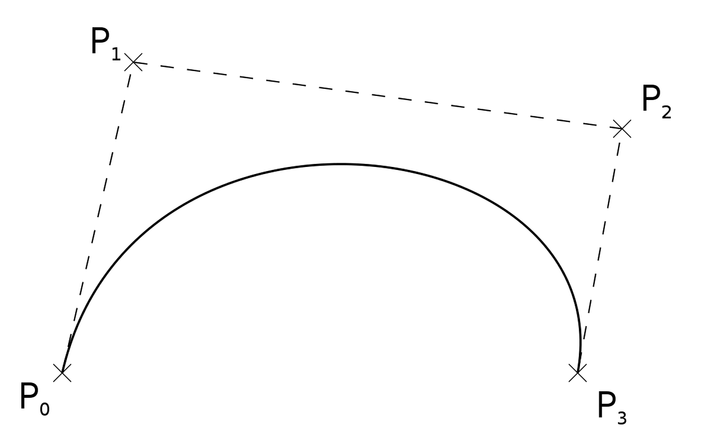 Cubic Bézier curve with four control points
Why Cubic Bezier?
Cubic bezier curves are the standard for custom timing functions because they offer:
- Smooth continuity: The curve is infinitely smooth with continuous derivatives
- Intuitive control: The control points provide predictable influence over the curve shape
- Computational efficiency: Fast evaluation makes them perfect for real-time animation
- Universal support: Supported across all modern browsers and animation libraries
Popular easing functions like ease-in, ease-out, and ease-in-out are actually just predefined cubic bezier curves:
- ease-in-out:
cubic-bezier(0.42, 0, 0.58, 1) - ease-in:
cubic-bezier(0.42, 0, 1, 1) - ease-out:
cubic-bezier(0, 0, 0.58, 1)
Converting Custom Easing Functions
Let's say you have a custom easing function like a sharp quintic ease:
def ease_sharp(t):
    return t ** 5

# Generate 11 points from 0 to 1 (inclusive) and print normalized values
for i in range(11):
    t = i / 10.0  # Normalize input to [0, 1]
    result = ease_sharp(t)  # Compute eased value
    print(f"Input: {t:.1f}, Output: {result:.6f}")
This creates a very distinctive curve with slow initial movement and rapid acceleration toward the end. But how do we find the cubic bezier parameters that best approximate this behavior?
Introducing Delta Ease
The key to accurate conversion lies in defining what makes one approximation better than another.
Where:
Point-wise Error (
Derivative Error (
The derivative of our cubic bezier curve is:
Endpoint Error (
Where
The Optimization Process
With our error metric defined, we use numerical optimization to find the best cubic bezier parameters:
def guess_cubic_bezier(target_func, t_samples):
    def error(params):
        return delta_ease(target_func, params, t_samples)

    initial_guess = [0.42, 0.0, 0.58, 1.0]  # Start with ease-in-out
    bounds = [(-2.0, 2.0), (-2.0, 2.0), (-2.0, 2.0), (-2.0, 2.0)]

    result = minimize(error, initial_guess, bounds=bounds, method='L-BFGS-B')
    return result.x
The L-BFGS-B algorithm efficiently searches the parameter space, guided by
Real-Life Example
Let's apply this to our sharp quintic function
def sharp_quintic(t):
    return t ** 5
Here the complete implementation samples the function at 200 points between
import numpy as np

import matplotlib
matplotlib.use('agg')
import matplotlib.pyplot as plt

from scipy.optimize import minimize
from io import BytesIO
import base64

easing_functions = [
    ("sharp_quintic", lambda t: t**5),
    ("elastic", lambda t: -2**(10*(t-1)) * np.sin((t*10-0.75)*2*np.pi/3) if t < 1 else 1),
    ("bounce", lambda t: 1 - (7.5625*(1-t)**2 if (1-t) < 0.36363636 else
                              7.5625*(1-t-0.54545454)**2 + 0.75 if (1-t) < 0.72727272 else
                              7.5625*(1-t-0.81818181)**2 + 0.9375 if (1-t) < 0.90909090 else
                              7.5625*(1-t-0.95454545)**2 + 0.984375)),
    ("circular", lambda t: 1 - np.sqrt(1 - t**2))
]

def cubic_bezier(t, p0, p1, p2, p3):
    t2 = t * t
    t3 = t2 * t
    mt = 1 - t
    mt2 = mt * mt
    mt3 = mt2 * mt
    return p0 * mt3 + 3 * p1 * mt2 * t + 3 * p2 * mt * t2 + p3 * t3

def cubic_bezier_derivative(t, p0, p1, p2, p3):
    mt = 1 - t
    return 3 * (p1 - p0) * mt * mt + 6 * (p2 - p1) * mt * t + 3 * (p3 - p2) * t * t

def delta_ease(target_func, bezier_params, t_samples):
    x1, y1, x2, y2 = bezier_params
    target_values = np.array([target_func(t) for t in t_samples])
    bezier_values = np.array([cubic_bezier(t, 0, y1, y2, 1) for t in t_samples])
    point_diff = np.mean((target_values - bezier_values) ** 2)
    target_deriv = np.gradient(target_values, t_samples)
    bezier_deriv = np.array([cubic_bezier_derivative(t, 0, y1, y2, 1) for t in t_samples])
    deriv_diff = np.mean((target_deriv - bezier_deriv) ** 2)
    endpoint_weight = 10.0
    endpoint_diff = (target_func(0) - cubic_bezier(0, 0, y1, y2, 1)) ** 2 + \
                    (target_func(1) - cubic_bezier(1, 0, y1, y2, 1)) ** 2
    total_delta = 0.5 * point_diff + 0.3 * deriv_diff + 0.2 * endpoint_weight * endpoint_diff
    return total_delta

def guess_cubic_bezier(target_func, t_samples):
    def error(params):
        return delta_ease(target_func, params, t_samples)
    initial_guess = [0.42, 0.0, 0.58, 1.0]
    bounds = [(-2.0, 2.0), (-2.0, 2.0), (-2.0, 2.0), (-2.0, 2.0)]
    result = minimize(error, initial_guess, bounds=bounds, method='L-BFGS-B', options={'maxiter': 1000})
    return result.x

t_values = np.linspace(0, 1, 200)
plots = []

try:
    for name, func in easing_functions:
        original_values = [func(t) for t in t_values]
        x1, y1, x2, y2 = guess_cubic_bezier(func, t_values)
        control_points_x = [0, x1, x2, 1]
        control_points_y = [0, y1, y2, 1]
        bezier_values = [cubic_bezier(t, 0, y1, y2, 1) for t in t_values]
        delta_e = delta_ease(func, [x1, y1, x2, y2], t_values)

        plt.figure(figsize=(6, 6))
        plt.plot(t_values, original_values, label=f"{name} (Original)", color="blue")
        plt.plot(t_values, bezier_values, label=f"Guessed Bezier ({x1:.3f}, {y1:.3f}, {x2:.3f}, {y2:.3f})", color="red", linestyle="--")
        plt.plot(control_points_x, control_points_y, "go-", label="Guessed Control Points", alpha=0.5)
        plt.axhline(0, color='gray', linestyle='--', alpha=0.3)
        plt.axhline(1, color='gray', linestyle='--', alpha=0.3)
        plt.ylim(-1.5, 3)
        plt.title(f"{name} vs Guessed Cubic Bezier (eΔ = {delta_e:.4f})")
        plt.xlabel("t (time)")
        plt.ylabel("Output")
        plt.legend()
        plt.grid(True)

        buf = BytesIO()
        plt.savefig(buf, format='png')
        plt.close()
        plot = base64.b64encode(buf.getvalue()).decode('utf-8')

        print('data:image/png;base64,' + plot)

        print(f"{name} - Guessed cubic-bezier control points: ({x1:.3f}, {y1:.3f}, {x2:.3f}, {y2:.3f})")
        print(f"{name} - Delta Ease: {delta_e:.4f}")
except Exception as e:
    print(f"Error generating plots: {str(e)}")
The resulting closely approximates the curves of the original easing functions, with the
Practical Applications
This technique opens up possibilities for:
- Design System Consistency: Convert brand-specific easing curves to CSS-compatible format
- Physics-Based Animation: Approximate complex physical simulations with simple bezier curves
- Cross-Platform Compatibility: Ensure consistent timing across different animation libraries
- Performance Optimization: Replace expensive mathematical functions with efficient bezier evaluation
Conclusion
Converting arbitrary easing functions to cubic bezier curves bridges the gap between mathematical creativity and practical implementation. By combining point-wise accuracy, derivative matching, and endpoint precision in our Delta Ease metric, we can faithfully approximate complex timing functions with the universally-supported cubic bezier format.
This approach democratizes custom animation timing, making sophisticated easing curves accessible to any developer working within the constraints of standard web technologies.